Part I - Using R in Excel - Descriptive Statistics

Introduction

The purpose of this series of posts is to demonstrate some use-cases for R in Excel using the ExcelRAddIn component (disclaimer: I am the developer of this add-in: ExcelRAddIn). The fundamental rationale for the add-in is that it allows access to the extensive R ecosystem within an Excel worksheet. Excel provides many excellent facilities for data wrangling and analysis. However, for certain types of statistical data analysis, the limitations of the built-in functions even alongside the Analysis ToolPak is not sufficient, and R provides superior facilities (for example, for performing LDA, PCA, forecasting and time series analysis to mention a few).

This series of posts demonstrates four main areas where R is useful in Excel: descriptive statistics, linear regression, forecasting, and accessing Python. Along the way, we will see that using R in Excel is no more difficult than writing a formula and calling the ExcelRAddIn to evaluate it. The ‘trick’, if there is one, is unpacking the results into a form that Excel understands and which can be used in a worksheet. We will see several examples of how to do this.

Installing and setting up the ExcelRAddIn is described here. Each part of the series is accompanied by an Excel workbook with the R scripts. The workbooks depend on the ExcelRAddIn-AddIn64.dll, so this should be loaded first, and the “R AddIn” menu should appear on the right-hand side of the menu bar.

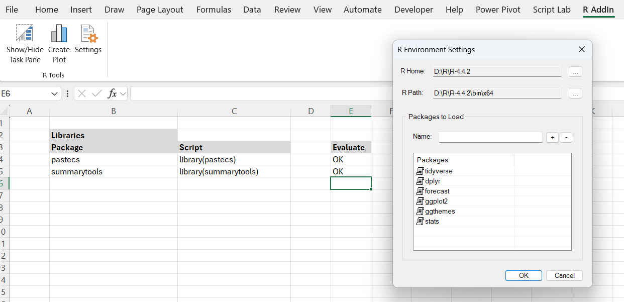
The task pane is empty until the first script is evaluated. This will initialise R using the directories in the “Settings”. The default packages I use are tidyverse, dplyr, forecast, ggplot2, ggthemes, as shown below:

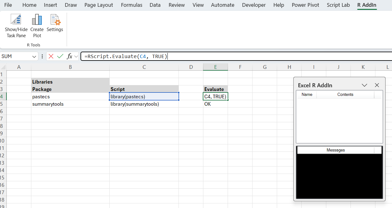
The workbook for this part of the series is: Part I - R in Excel - Descriptive Statistics.xlsx. The workbooks all have a similar structure just to keep things organised. The ‘References’ worksheet lists any links to external references. The ‘Libraries’ worksheet loads additional (non-default) packages. The ‘Datasets’ worksheet contains any data referenced in the worksheets.

Descriptive statistics

Loading Data

The first step is to load some data. This dataset comes from “Linear Models with R” by Julian Faraway. In this example, I have loaded the data into Excel from a csv file (GalapagosData.csv) using Power Query. The data has been tidied up and I have created a table (tableGalapagos) that can be referenced in the workbook.

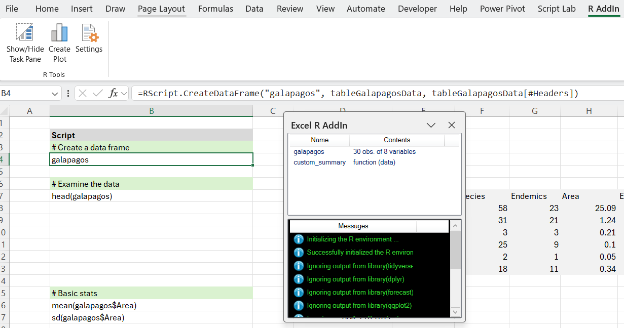
In the Descriptive Statistics worksheet, we first create a data frame using the CreateDataFrame function.

=RScript.CreateDataFrame("galapagos", tableGalapagosData, tableGalapagosData[#Headers])

This function is part of the add-in and simplifies the creation of dataframes. There are also functions to create vectors and matrices. We pass in a name (which will appear in the R environment) and the data and headers. The final parameter (‘Type’ => character, complex, integer, logical, numeric) is optional; the RType is now determined from the data if possible. This makes it somewhat easier to create objects to pass to R from Excel.

This copies the data into the R environment. There are a number of alternatives to this approach. We could have loaded the csv file directly into R using:

galapagos <- read.csv("D:\Development\...\GalapagosData.csv")

By loading the data into Excel and then copying it to R, we can leverage the Excel import using Power Query, so we automatically get grouping, filtering etc, and can immediately create PivotTables. The downside is that we need to make a copy into R, and this means ensuring the data types are ‘viable’. This is particularly important with dates.

Obtaining Statistics

Now that we have the data frame in R (and in Excel), we can obtain some descriptive statistics. If we were doing this exclusively in Excel, we might use individual formulas (=COUNT(), =AVERAGE(), =STDEV.S() and so on). Using R, we can accomplish the same thing.

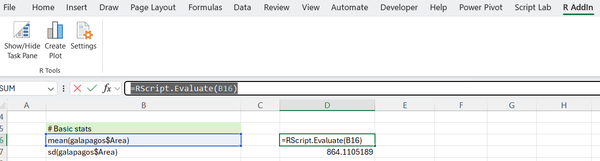
As expected, this returns the mean and standard deviation.

We can improve on this using some additional R functions: sapply together with fivenum (fivenum returns Tukey’s five number summary (minimum, lower-hinge, median, upper-hinge, maximum) for the input data).

as.data.frame(sapply(galapagos[,2:8], fivenum))

When evaluated, all this does is to apply the fivenum function to columns 2 to 8 (zero-based) of the galapagos dataset, and coerce the result into a dataframe. If we don’t do this we don’t get back the column headings (which is not tremendously useful). You may also have noticed that we have to determine the return values from the documentation. There doesn’t seem to be a way of retrieving this meta data from the function.

An alternative to the five-number summary is to use the built-in summary(...) function. Unfortunately the output from this does not work well with Excel, so we need to massage the results in order to obtain a decent table showing the summary with labels.

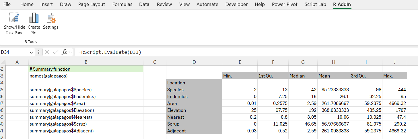
Basically, we get the column labels from the galapagos dataset using: names(galapagos), and we get the labels for the summary using: names(summary(galapagos$Species)). Then for each column of the data we are interested in, we request the summary. For example: summary(galapagos$Elevation).

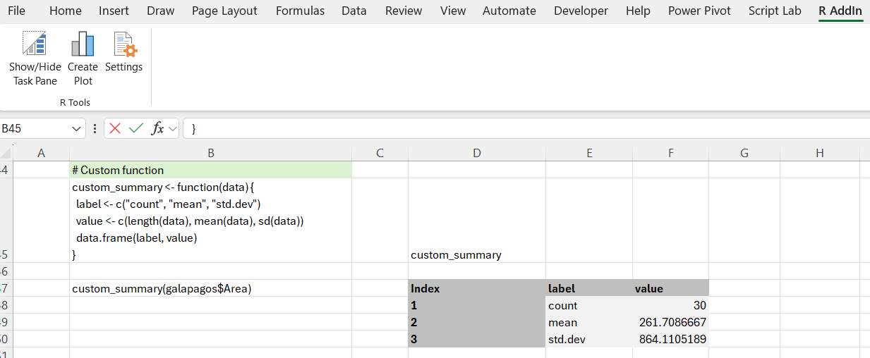
Now that we are massaging the results, we might even consider using a custom function. We can, for example, define a function that returns a dataframe consisting of a label and the corresponding statistic:

custom_summary <- function(data) {
  label <- c("count", "mean", "std.dev")
  value <- c(length(data), mean(data), sd(data))
  data.frame(label, value)
}

Evaluating the function with the script:

custom_summary(galapagos$Area)

outputs a small table, as follows:

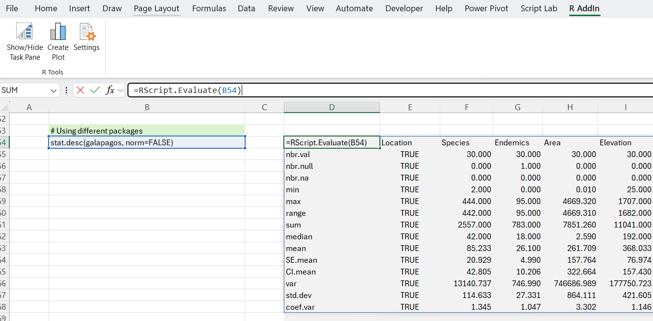
If all this seems quite a lot of hard work, or you are looking for a more sophisticated approach - perhaps a summary that tests the normality of the distribution of the data - then you might prefer to use a summary function from a different package. There are several to choose from. Here we use pastecs pastecs and summarytools summarytools. Both of these give good results with minimal effort:

Wrap up

In this post, we have seen various approaches to obtaining descriptive statistics using R in Excel via the ExcelRAddIn. We have introduced some basic approaches (similar to what Excel natively offers). But we have also seen some more advanced usage that demonstrates how useful it can be to have access to R functionality in Excel. The next post covers linear regression using R in Excel.