Part V - Using R in Excel - Inferential Statistics

Introduction

In the previous posts in this series (Using R in Excel) I have demonstrated some basic use-cases where using R in Excel is useful. Specifically we have looked at descriptive statistics, linear regression, forecasting, and calling Python. In this post, I am going to look at inferential statistics and how R can be used (in Excel) to perform some typical statistical tests. Excel provides many excellent facilities for data wrangling and analysis. However, for certain types of statistical data analysis the limitations of the built-in functions and the Analysis ToolPak is not sufficient, and R provides superior facilities.

The workbook for this part of the series is: “Part V - R in Excel - Inferential Statistics.xlsx”. As before, the ‘References’ worksheet lists links to external references. The ‘Libraries’ worksheet loads additional (non-default) packages. In this demonstration, I use ggpubr and the lsr package. The ggpubr package provides some easy-to-use functions for creating and customizing ‘ggplot2’-based publication ready plots. The lsr package provides some useful wrappers for common hypothesis tests and basic data manipulation. These packages should be present and loaded before continuing with the analyses.

The ‘Datasets’ worksheet contains the data referenced in the worksheets. The data for the main analyses represents the weights (in Kg’s) of 9 women and 9 men. The data has been loaded and an Excel table created named tWeightData.

Analysis I

Creating the data frame

The first thing to do is to create an R data frame. However, rather than having a table with two columns (women_weight and men_weight) we want a ‘Group’ column and a ‘Weight’ column. To do this we first create vectors using:

=RScript.CreateVector('women_weight',Datasets!N2:N10)

and

=RScript.CreateVector('men_weight',Datasets!O2:O10)

After this, we create the data frame specifying the grouping factors and the data. The corresponding vectors and the weight_data data frame should appear in the Excel R AddIn panel.

Comparing Means

The first analysis checks whether there’s a significant difference in the weights of the different groups. For this, we perform an independent samples t-test. Prior to performing the test, it is useful to provide a summary of the data, so we group the data to obtain the means and standard deviations, and we also produce a boxplot.

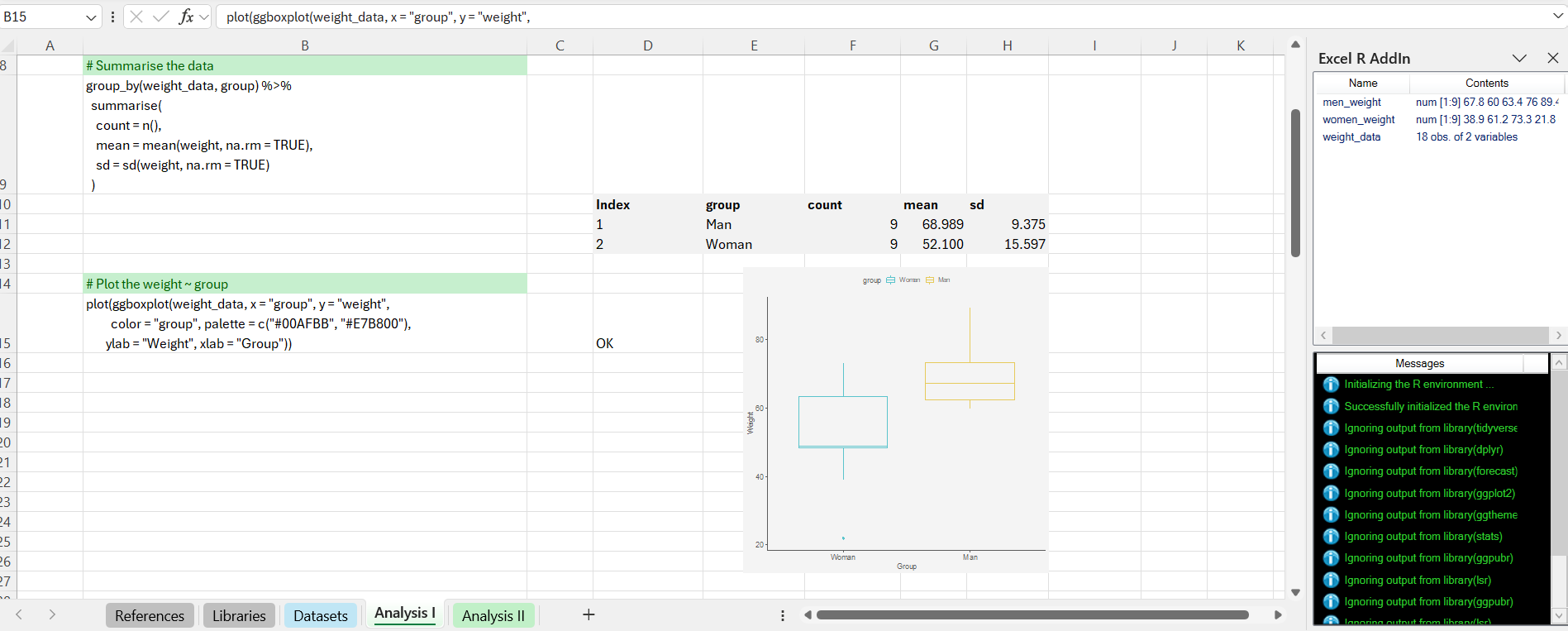
From the plot, there seems to be a plausible difference in the means. It is worth noting in passing that we use the standard ggboxplot(...) function, but wrap it in a call to the plot(...) function. This outputs the result to a separate graphics window, from which we can paste the resulting graphic as a Windows metafile. This is not ideal, but as yet I have not found a way to draw a plot directly in an Excel worksheet.

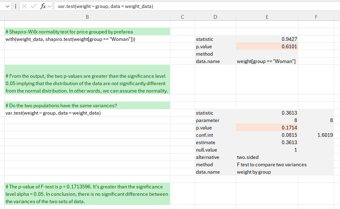
Before doing the t-test we want to check the independent t-test assumptions. Specifically, the two samples are independent since the observations come from distinct groups (men and women). We also want to check that the data from each of the groups follow a normal distribution. We perform a Shapiro-Wilk normality test for each group. We could also have inspected the data visually with a histogram or a qqplot.

From the output of the Shapiro-Wilk test, the two p-values are greater than the significance level 0.05 implying that the distribution of the data are not significantly different from the normal distribution. Therefore, we can assume the observations from each group follow a normal distribution.

Comparing Variances

In addition to the Shapiro-Wilk test, we perform an F-test to compare variances since one of the assumptions of a t-test is that the population variances should be equal. The output of var.test is a list containing the individual results, which we display. The p-value of F-test is p = 0.17136. Since it is greater than the significance level (alpha = 0.05) we conclude that there is no significant difference between the variances of the two sets of data. Therefore, we can use the classic t-test which assume equality of the two variances.

Unpaired two-samples t-test

Finally, we compute an independent t-test. As before, we extract the individual statistics. The p-value of the test is 0.01327, which is less than the significance level (alpha = 0.05). We can conclude that men’s average weight is significantly different from women’s average weight in this dataset with a p-value = 0.01327.

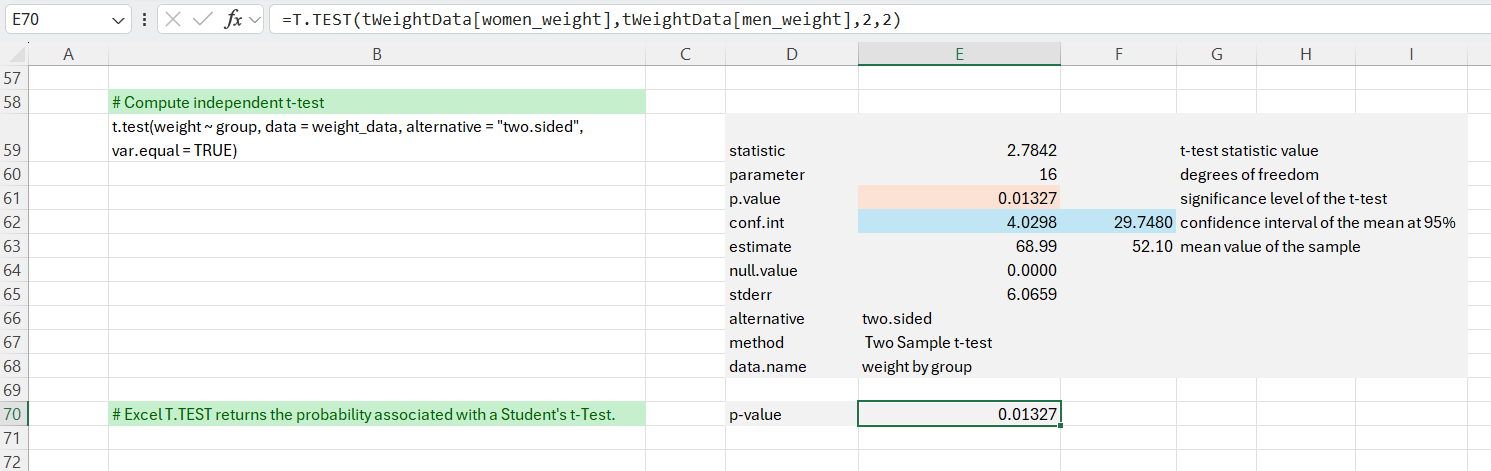
We can also check that Excel’s =T.TEST() function produces the same result.

Analysis II

One-way ANOVA

For the second analysis, we want to perform a one-way ANOVA test. We use the built-in R data set named PlantGrowth. It contains the weight of plants obtained under a control and two different treatment conditions.

As before, we display a brief summary of the data and a boxplot to visually display the means of each group. Then we compute the one-way ANOVA. The output contains a lot of data, so we extract the individual components as required.

We can also use the anova function to summarise the test results.

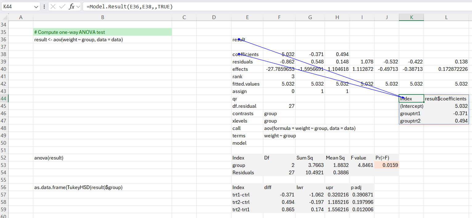
As the p-value is less than the significance level 0.05, we can conclude that there are significant differences between the groups.

Because the test result is significant, we compute Tukey HSD for performing multiple pairwise-comparison between the means of groups. It can be seen from the output, that only the difference between trt2 and trt1 is significant with an adjusted p-value of 0.012. The same test can be performed using Excel’s Analysis ToolPak ‘Single Factor ANOVA’ function. This is demonstrated in the ‘Single Factor ANOVA’ worksheet.

Wrap Up

In this post we have used R in Excel to perform some basic tests for inferential statistics. We have performed a Shapiro-Wilk test, an F-test, an independent samples t-test and a one-way ANOVA. In passing, we have also seen how to plot data and how to set up and retrieve model results. While some of this could have been done using Excel’s native functions, the advantage of using R from within Excel is that it gives us access to an extensive ecosystem, which in turn gives us a good deal of flexibility in creating solutions.