Part III - Using R in Excel - Forecasting

Introduction

We have already seen how to obtain descriptive statistics in Part I and how to use lm() in Part II. In this part (Part III) of the series we will look at using R in Excel to perform forecasting and time series analysis.

In the previous two parts we have seen different ways to handle the output from R function calls, unpacking and massaging the data as required. In this part we are going to focus on setting up and interacting with a number of models in the ‘forecast’ package (fpp2).

The workbook for this part of the series is: “Part III - R in Excel - Forecasting.xlsx”. As before, the ‘References’ worksheet lists links to external references. The ‘Libraries’ worksheet loads additional (non-default) packages. In this demonstration, I use the fpp2 package. The ‘Datasets’ worksheet contains the data referenced in the worksheets.

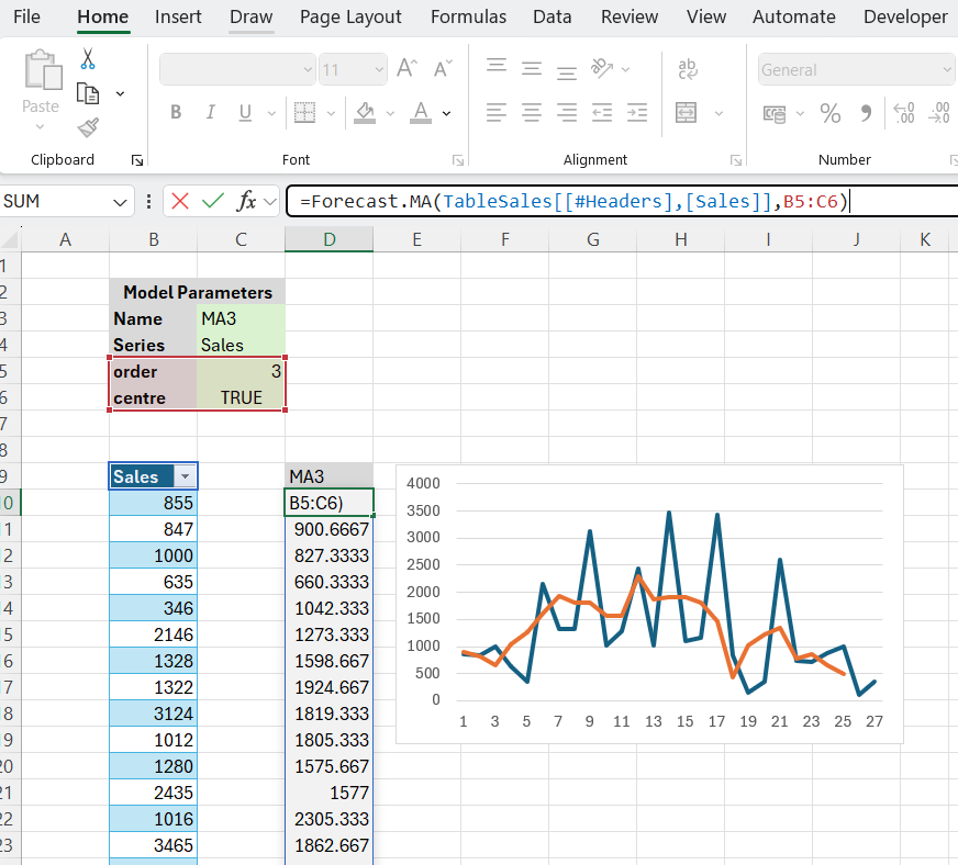
Moving Average

In this worksheet we are looking at the moving average function in the forecast package. ma computes a simple moving average smoother of a given time series. The data we use consists of ice cream sales.

In the previous posts we have used ‘scripts’ to call R functions. So, in this case we could evaluate

ma(Sales, 3, FALSE)

and get back the smoothed time series.

However, as the models become more complex, and the number and types of parameters increases, this approach becomes less manageable. An alternative is to use one of the custom Forecast. functions provided by the add-in. This allows us to set up the model parameters as a block of named parameters with their corresponding values. We have already seen an example of this in Part II where we set up a logistic regression model. In the case of Forecast.MA, we give the model a descriptive name. We know from the documentation that the model takes two parameters: the order (“order of moving average smoother”) and the center (“if TRUE, then the moving average is centred for even orders”). Then we just call a regular Excel worksheet function.

The add-in provides wrappers around a number of the functions in the forecast package. These are as follows:

• Forecast.MA - Moving average smoothing
• Forecast.SES - Simple exponential smoothing
• Forecast.Holt - Holt exponential smoothing
• Forecast.HW - Holt-Winters exponential smoothing.
• Forecast.AutoETS - Exponential smoothing state space model.
• Forecast.Arima - Auto-Regressive Integrated Moving Average model
• Forecast.AutoArima - Fit best ARIMA model to univariate time series
• Forecast.FC - Generic function for forecasting from time series or time series models
• Forecast.meanf - Mean forecast
• Forecast.rwf - Forecasts and prediction intervals for a random walk with drift model
• Forecast.splinef - Local linear forecasts and prediction intervals using cubic smoothing splines
• Forecast.thetaf - Forecasts and prediction intervals for a theta method forecast
• Forecast.Croston - Forecasts and other information for Croston’s forecasts

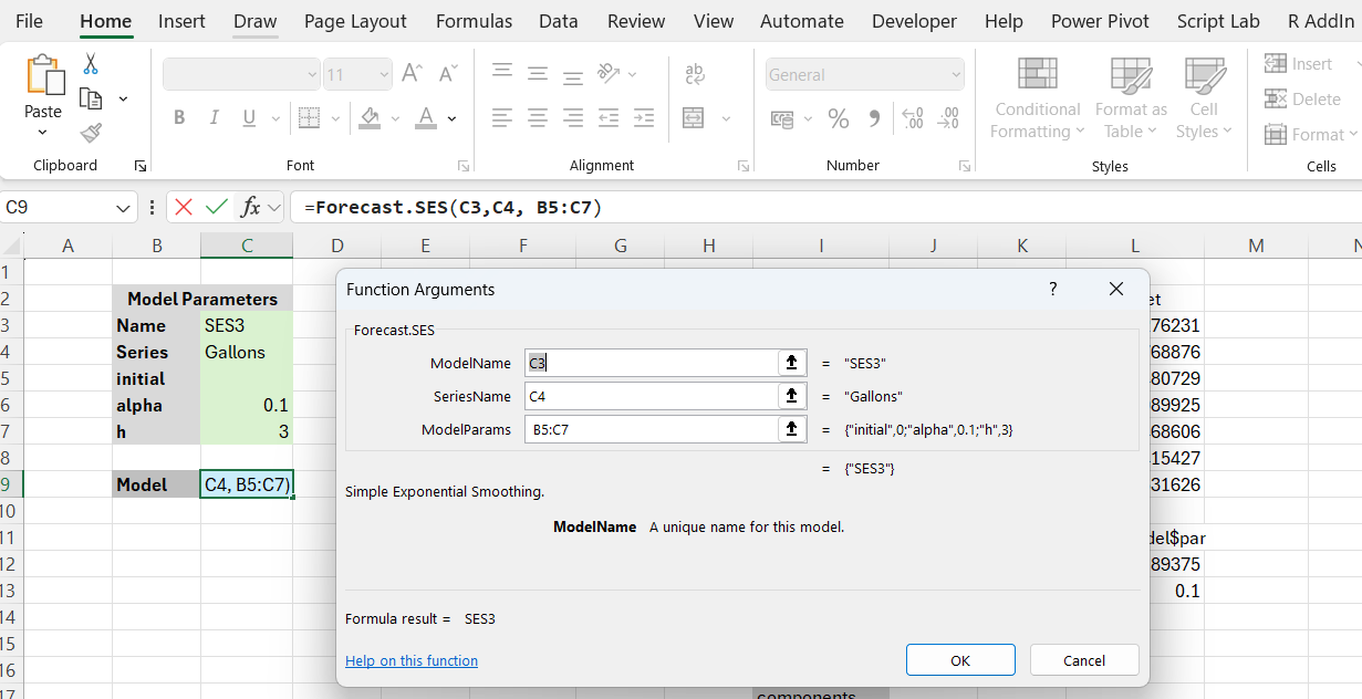
Simple Exponential Smoothing

In this example, we create a simple exponential smoothing model. As before we set up the model parameters following the forecast package ses documentation. Fortunately, most of the values are defaulted so we only provide inputs for the following:

• alpha - the value of the smoothing parameter for the level. If NULL, it will be estimated.
• h - the number of periods for forecasting.

Then we can call the add-in function Forecast.SES(...).

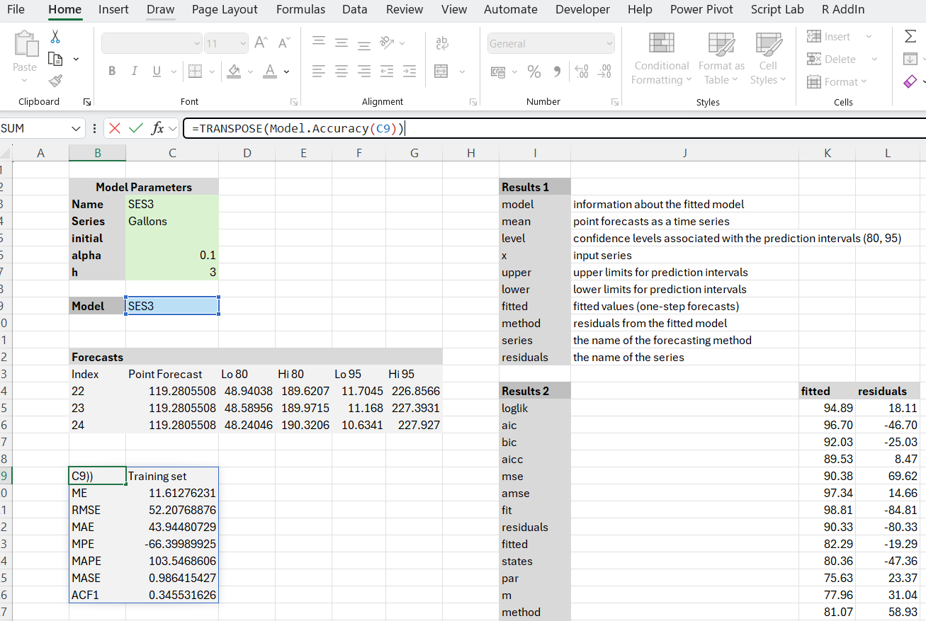
The model returns the requested forecasts with the mean, and lower and upper limits for the prediction intervals.

In previous examples, we have extracted model results by concatenating the returned model name (‘SES3’ in this case) with labels from the model. As illustrated in Part II, in order to make it easier to retrieve results, the add-in provides some additional functions for querying models: Model.Results outputs a list of results from the model. Model.Result outputs the result obtained from one item of the list of model results. Optionally, the result can be formatted as a data frame. This is somewhat more convenient than having to evaluate scripts of the form model name'$coeffcients, etc. Finally, Model.Accuracy returns a number of statistics relating to measures of model accuracy.

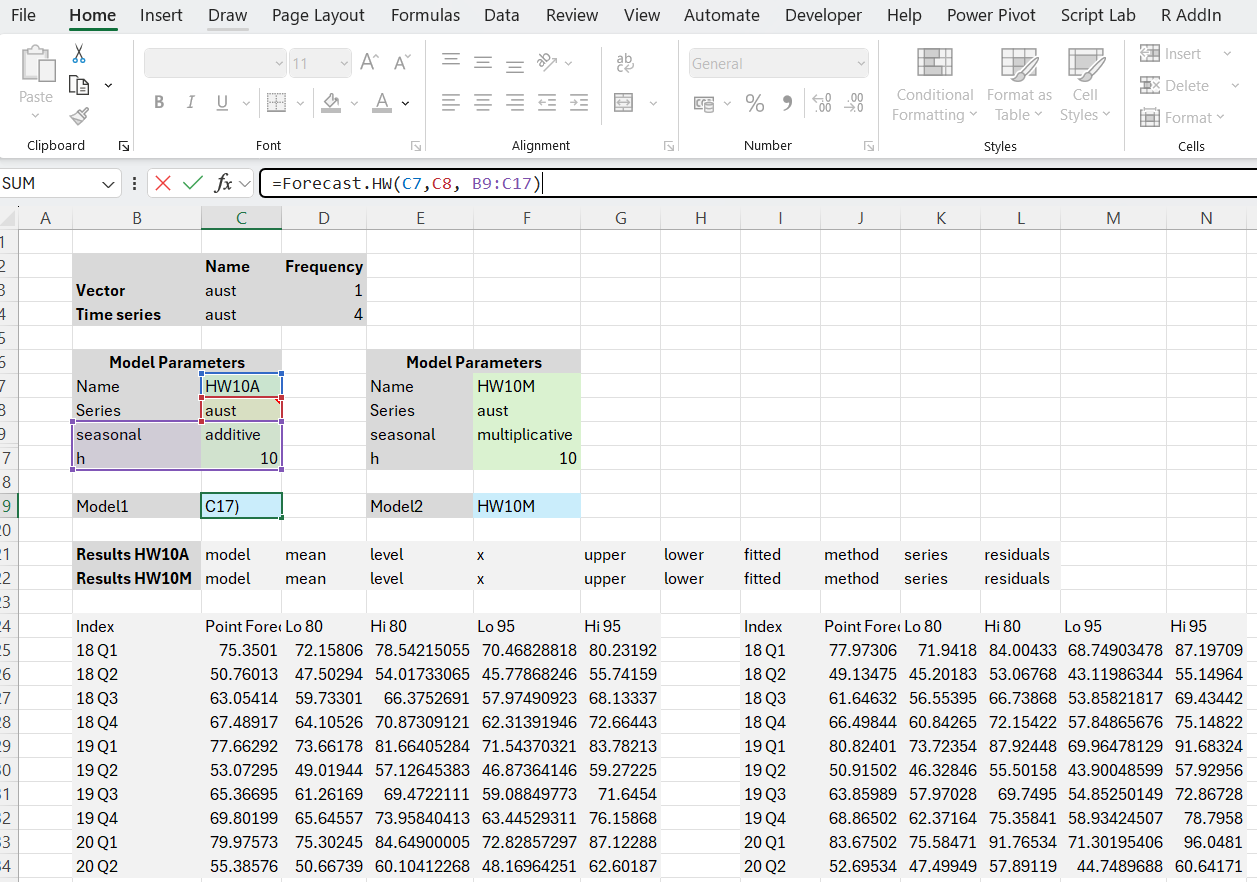
The Holt-Winters model

The HW worksheet illustrates working with the Holt-Winters model. In this case, we set up two different models with their respective parameters, each with their own parameter block: an additive model and a multiplicative model. However, we first need to address an issue with the ‘data type’ of the dataset. Typically we can just create a numeric vector. Unfortunately, the series parameter of the Holt-Winters model requires information about the frequency with which the observations in the vector occur. Therefore we create a numeric vector first and then convert it into a ts time-series vector with embedded frequency information. Currently, the ExcelRAddIn does not support time series as a data type. This will be added as a future enhancement.

ARIMA

The final example concerns the ARIMA model. The setup of the model is somewhat more complicated than in previous cases. Specifically, the order and the seasonal parameters.

From the documentation we know that the order parameter is a specification of the non-seasonal part of the ARIMA model: the three components (p, d, q) are the AR order, the degree of differencing, and the MA order. To handle this specification, we input the components using the vector notation: c(0, 1, 1).

For the seasonal parameter, the documentation says: “A specification of the seasonal part of the ARIMA model, plus the period (which defaults to frequency(y)). This should be a list with components order and period, but a specification of just a numeric vector of length 3 will be turned into a suitable list with the specification as the order.”

To achieve this we add a script parameter. This is a parameter with a leading ‘^’ character as follows:

^list(order=c(0,1,1),period=12)

With this setup we can create the ARIMA model.

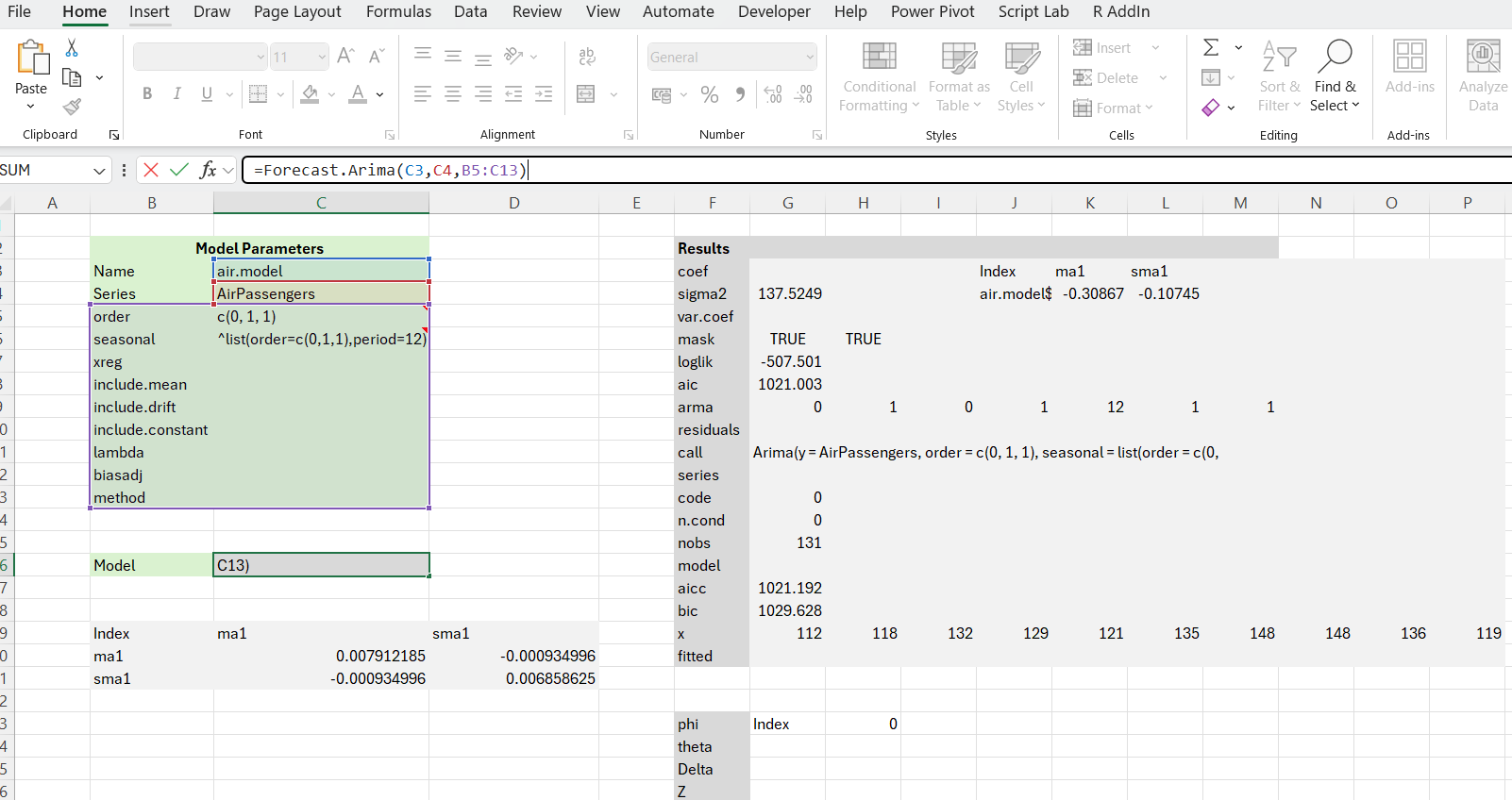
The results can be extracted using a combination of Model.Results and Model.Result functions or by using a ‘raw’ R script. The model accuracy can be checked via the function Model.Accuracy(...).

Wrap Up

In this post we have used R in Excel to perform some forecasting and time series analyses. We have seen how to set up and retrieve model data. In addition to evaluating R scripts, we have also made use of a number of wrapper functions around the Forecast package provided by the add-in to make model setup and evaluation easier.

In the last part of the series I will look at using R in Excel to call Python scripts.