Adventures in Excel: Filtering and grouping data

Introduction

This started off as a simple experiment and mushroomed (a little). I have a card account, and I wanted to know how much I owed for the previous and current month. Simple enough. And it was, until I started to think about different possible ways to do this. In this post I describe five different approaches that answer the question: “How much do I owe in May, Jun, Jul, etc.?” The spreadsheet can be downloaded from here: AccountQueries.xlsm

The data

The data consists of a list of card transactions with the date and some details. It is defined as an Excel table named ‘TableTransactions’. This makes it easy to reference in formulas and functions requiring a named range/table. The columns of interest here are the ‘Date’ (specifically the month) and the (sum of) the ‘Withdrawal’ column: i.e. how much is owed for that month.

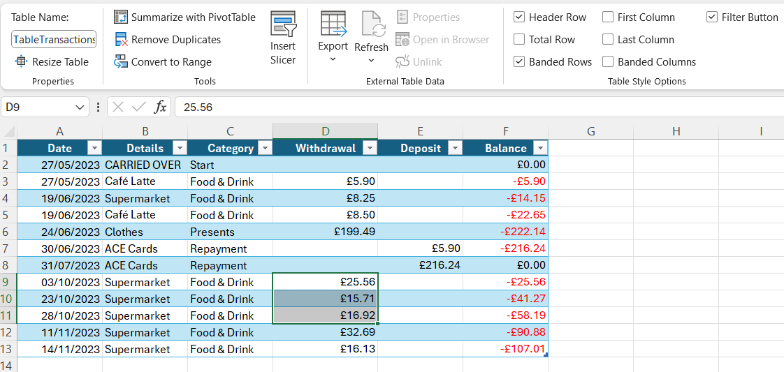
To answer the question “How much do I owe?” we could adopt a manual approach and simply select the cells we want to sum (as in the screenshot). This works, but is not reusable and not great when you have more data. I was looking for approaches that would work as the data is extended. This is what I came up with.

1. An Excel Formula

Using an Excel formula is the simplest and most obvious approach. Despite this simplicity, the formula is a little involved: =SUM(CHOOSECOLS(FILTER(TableTransactions,TEXT(TableTransactions[Date],"mmm")=B3, 0),4)).

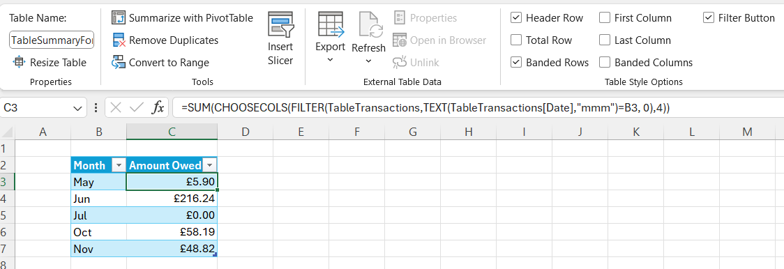
Starting with the innermost formula and working outwards: TEXT(TableTransactions[Date],"mmm") takes the date and extracts the (short) month part of the date as text. This is compared to the input month (ignoring months where we haven’t spent anything). This condition is part of the FILTER formula, which returns all the rows from TableTransactions where the condition is met. We only want the ‘Withdrawal’ column, so we restrict the filtered results using CHOOSECOLS to select column 4 as the column of interest. Finally, we use SUM to aggregate the amounts in this column. There are several variations of this approach using other Excel formulas (e.g. XLOOKUP, INDEX, and MATCH). However, this formula answers the question we wanted.

2. A Lambda Expression

This is an extension of the previous approach. We can write an expression using LAMBDA which takes a single parameter - the short month name - and passes it to the SUM(CHOOSECOLS(...)) formula and evaluates it. Furthermore, we can give this a name like AmountOwedLambda(...) using the Name Manager.

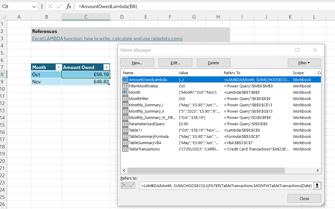
Now we have a reusable named function, which seems quite neat. However, it is still rather opaque when you view the formula in the Name Manager.

3. A Pivot Table

In some ways using a pivot table seems the most natural Excel-way to summarise the data. It is very simple to create. Select Insert > PivotTable > From Table/Range. For the rows, we select Months and for the Values we sum the ‘Withdrawal’ column - which we rename to ‘Amount Owed’.

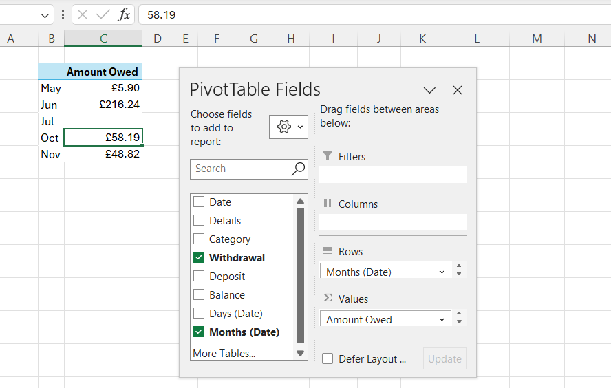
That is all there is to it. This is really simple and extends well for other months (and other dates).

4. A Power Query

Rather than use a PivotTable to summarise the data, we can use PowerQuery. There are (at least) two variations on this. The first is simply to specify the filter/group clauses in PowerQuery. This is done in ‘Monthly Summary I’. The exact steps are recorded in M-language statements. In this case, we clean up the Date column to produce a column with a short month name, and then group by that month. In a custom column we sum by the ‘Withdrawal’ column. Once we have finished defining the steps, we get back a table in a worksheet.

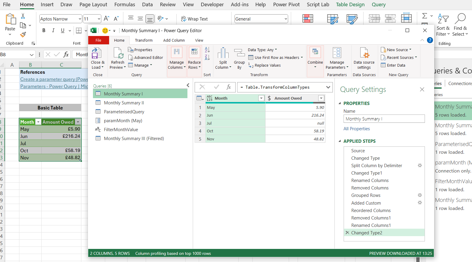
The results are more or less the same as with the Pivot Table. Any updates to the original transactions table are reflected in the ouput of the PowerQuery after doing a refresh.

The second approach is to prepare a filtered query. This is somewhat fiddly. First you need a table (or a named range) representing the input parameter. Once this is defined in PowerQuery, put it to one side. Then define the PowerQuery like the basic table but filtered with a hardcoded month. Finally, edit the M language query to use the input parameter in the query instead of the hardcoded month.

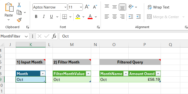
In the worksheet, we just enter a month and press refresh, and the results are returned. Full details about how this is set up are given in the references section of the worksheet.

5. A VBA Function

One final approach is to write a VBA function. For this we need to create a VBA project, add a module that contains the code, and save the file as a macro-enabled workbook. This may seem like overkill for what I orginally wanted. However, there are some advantages. It is flexible, allowing us to decide how to treat the input - in this case converting a short month name to a month number - and it allows us to break down the parts of the formula into a loop (for better or worse).

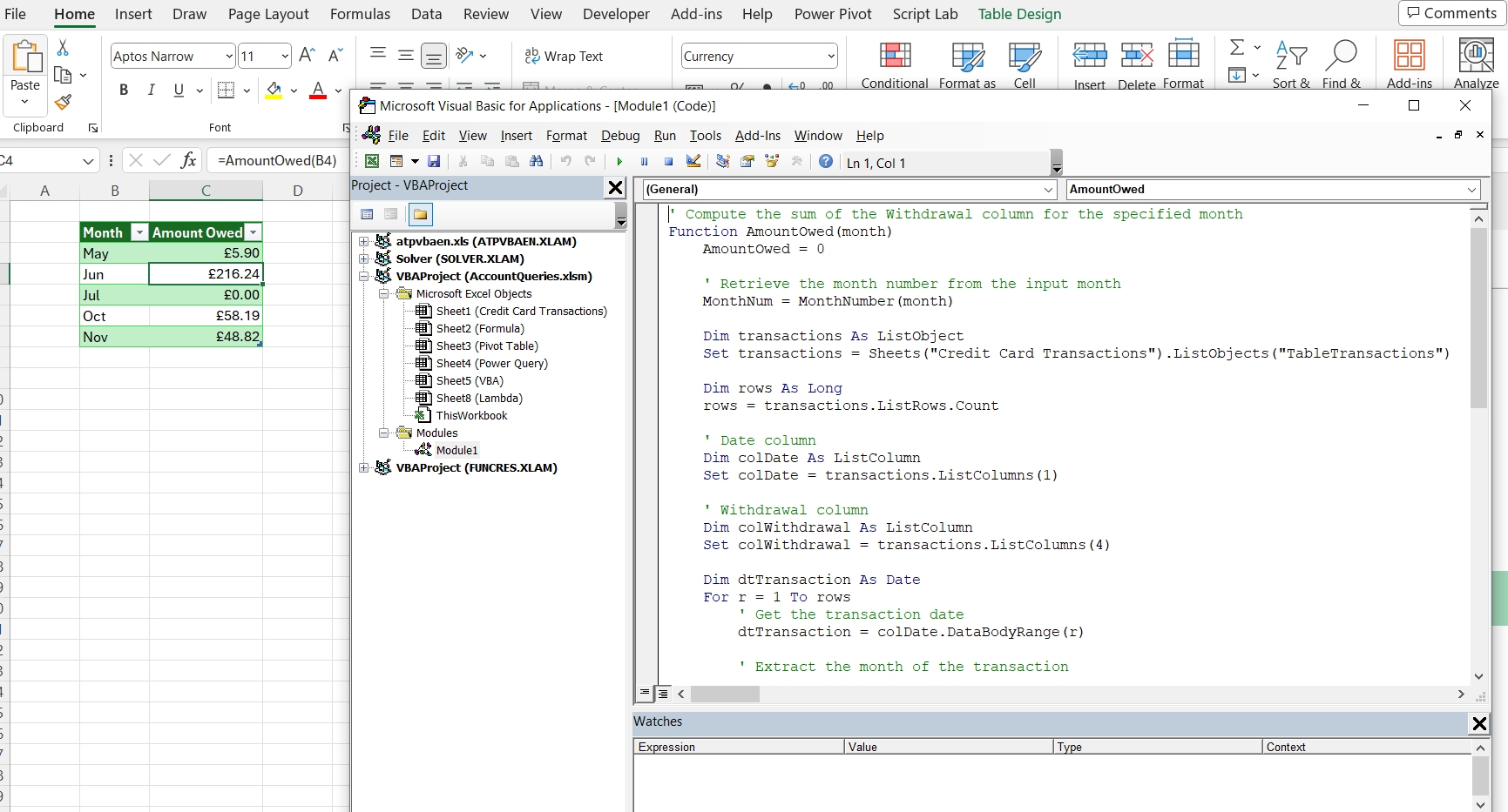
It is also useful in that the function (the code) is reasonably well-documented.

Wrap up

So there it is. Five ways to achieve pretty much the same thing in Excel: Excel formulas, a custom Lambda, a pivot table, PowerQuery and finally VBA. Each has advantages and drawbacks. But it doesn’t stop there. We could just as easily use SQL, or perhaps even better, PowerPivot and a DAX query. And for a really over-the-top solution, we could consider using the excellent Excel-DNA library to write a user-defined function in C#.